Meaning chains with word embeddings

Matthew Lincoln recently put up a Twitter bot that walks through chains of historical artwork by vector space similarity. https://twitter.com/matthewdlincoln/status/1003690836150792192.
The idea comes from a Google project looking at paths that traverse similar paintings.

This reminds that I’d meaning for a while to do something similar with words in an embedding space. Word embeddings and image embeddings are, more or less, equivalent; so the same sorts of methods will work on both. There are–and will continue to be!–lots of interesting ways to bring strategies from convoluational image representations to language models, and vice versa. At first I though I could just drop Lincoln’s code onto a word2vec model, but the paths it finds tend to oscillate around in the high dimensional space more than I’d like. So instead I coded up a new, divide and conquer strategy using the Google News corpus. Here’s how it works.

1. Take any two words. I used “duck” and “soup” for my testing.
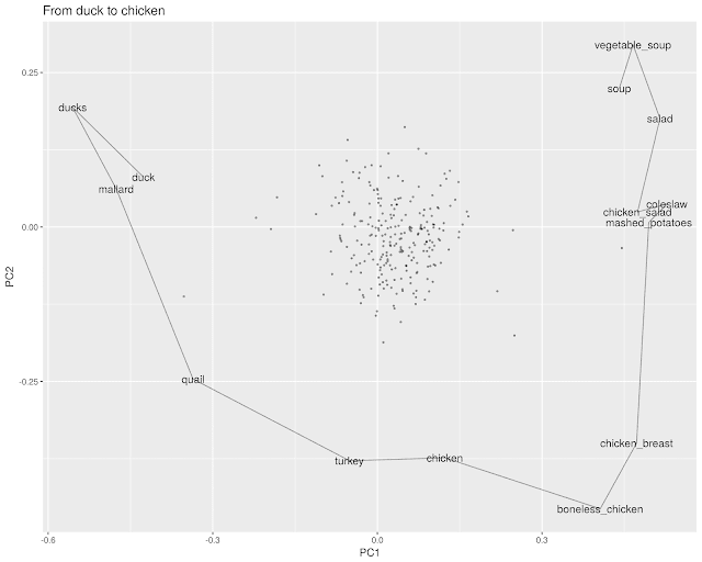
2. Find a word that is, in cosine distance, *between* the two words: that is, that is closer to both of them than either is to each other. Select for one as close to the midpoint as possible.* With “duck” and “soup,” that word turns out to be “chicken”: it’s a bird, but it’s also something that frequently shows up in the same context as soup.
3. Repeat the process to find words between “duck” and “chicken.” That, in this corpus, turns out to be “quail.” The vector here seems to be similar to the one above–quail is food relatively more often than duck, but less overwhelmingly than chicken.
4. Continue subdividing each path until no more intermediaries exist. For example, “turkey” works as a point between “quail” and “chicken”; but nothing intermediates between turkey and quail, or between turkey and chicken.

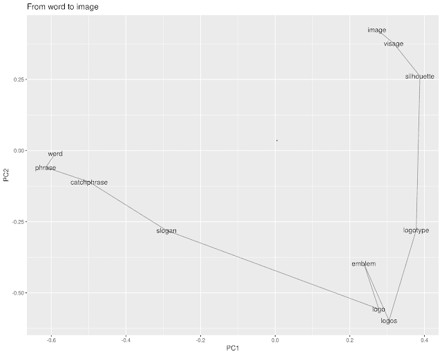
The overall path then sketches out an arc between the two words. (The shape of the arc itself is a component of PCA, but it’s also a useful reminder that the choice of the first pivot is quite important–it sets the entire region for the rest of the search.

(I put a few random words as unlabelled dots in the background–this should serve mostly as a reminder of how odd the geometries of high-dimensional spaces are. With any of these paths, even between relatively similar words, it’s not hard to find a perspective where they appear to be on opposite ends of the full galaxy of language).

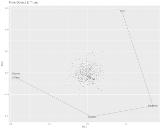
As with any method, this can be somewhat useful as a way to start understanding the contents of the vectorspace being used. How, for example, do you get from “Trump” to “Obama?” Google News is mostly from almost a decade ago, so the answer lies primarily in New York state. Hillary Clinton has stronger connections to the New Yorkers, and Rudy Giuliani serves as a proto-Trump in that space. Between Trump and Giuliani, interestingly, is the Tea Party 2010 GOP NY gubernatorial nominee Carl Paladino (I had not though about that name in a quite a while!) who seems to serve as a kind of bridge between whatever Trump was doing in 2011 and the GOP establishment, such as it was.

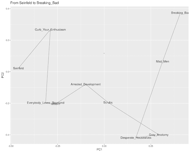
As this suggests, there’s a certain kind of deep cultural knowledge built into the co-occurrence networks of news articles that word2vec trains on. The path from “Seinfeld” to “Breaking Bad,” for example, initially realizes that “Curb Your Enthusiasm” mediates between the 90s show and the Golden Age of television; and then sets about bridging the drama-comedy divide by finding its way into the primetime soaps through “Scrubs” out of the comedies and “Mad Men” out of the dramas.
There are some odd choices–“Everybody Loves Raymond” and the raw word “sitcom” seem unnecessary to mediate between “Curb” and “Arrested Development,” but in general the paths are interesting, at least.

Other times, they simply suggest connecting angles. From “word” to “vector” moves through rasters and parsers to kiss in the land of .dll files. How supremely unlovely.

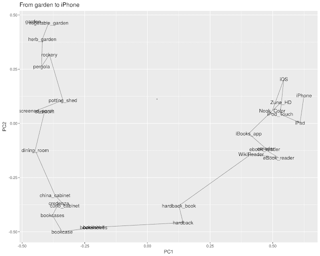
Occasionally the paths get downright baroque–this, I think, has to do with the oddness of using cosine similarity to interpolate, which makes it relatively easy to find intermediate points.** The path from “iPhone” to “garden,” for example, takes a wonderfully evocative path through the cultivated landscape (“rockery”, “pergola”) into a home (“dining room”, “china cabinet”, “bookcases”) and upon pulling a “hardback book” off the shelf abruptly shifts into the digital age through e-readers and forgotten formats (remember the Zune?) before landing at the iPad.

This enterprise is more evocative than useful, except in that it gives another way to understand the vector models that are an increasingly important part of the information architecture of modern life. Looking at them reminds me in an odd way of the way I was taught to read poetry in high school and college, in two senses.

The first is that it relies heavily on the ability of individual words to conjure up their surroundings. The left half of the above chart pleases (if it does) because, for example, “rockery” is such a rare and specific word–it lives primarily in the world of Beatrix Potter. The whole path to the bookcases past the credenza, above, brings to mind the small soul in the window seat in TS Eliot’s Animula. The second part *doesn’t* please because the brands on the right have no weight or meaning on their own.

The second is the idea of the path itself. I was taught to read (short) poems as voyages that move in a direction; exteriority to interiority, personal to social, etc. It would be interesting to take individual poems and fit their direction to a general path in the overall vectorspace. This would provide a nice analogue to plot arceology for poems; are there particularly schemas especially present in certain genres? What are dissimilar poems that follow similar directional paths in different parts of the space?

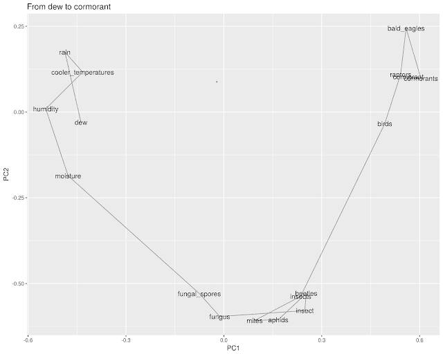
Or you could just use them to seed bad nature poems; start with a drop of dew, move out through the humidity to the mites and aphids, out to the raptors and cormorants.

*1: Math/high dimensional spaces note: This turns out to be an interesting problem that makes me wish I had taken some linear algebra at some point in my life. You might think you could simply find points that are close to the midpoint of the two words, but it’s almost always the case that the two words are closer to their midpoint than any other word. Similarly with differences

**It’s possible that a distance measure that satisfies the triangle inequality would work better; it’s also possible that what I really should do is manually choose between the top 5 pivot points, although I don’t want to do that on purely a useless thing that’s hard to build into a web app.

Comments:

I’m going to bury the code for actually doing …

Ben - Jun 3, 2018

I’m going to bury the code for actually doing this in the comments.

cpath = function(matrix, w1, w2, blacklist = c()) {
p1 = matrix[[w1]]
p2 = matrix[[w2]]

base_similarity = cosineSimilarity(p1, p2)
pairsims = matrix %*% t(rbind(p1, p2))
# Words closer to *either* candidate than the other word. These might be used eventually; mostly to save on computation in later steps.
decentsims = pairsims[apply(pairsims, 1, max) >= base_similarity[1],]
# Words closer to *both* candidates than the other word. The best of these is the intermediary.
greatsims = pairsims[apply(pairsims, 1, min) >= base_similarity[1],]
if (length(nrow(greatsims))==0 || nrow(greatsims) == 0) {
return(unique(c(w1, w2)))
}
pivot = order(-rowSums(greatsims))[1:4]
pivotwords = rownames(greatsims)[pivot]
pivotword = pivotwords[!pivotwords %in% c(w1,w2, blacklist)][1]
# highlight pivots.
message(w1, “<–>”, toupper(pivotword), “<—>”, w2)
if(is.null(pivotword) || is.na(pivotword)) {
message(w1,w2)
return(unique(c(w1, w2)))
}
pivotpoint = matrix[[pivotword]]

# Really, this should *different* for the right and left side.
mat = matrix[rownames(matrix) %in% rownames(decentsims),]

left = cpath(mat, w1, pivotword, blacklist = c(w1, w2, blacklist))
right = cpath(mat, pivotword, w2, blacklist = c(w1, w2, blacklist))
return(unique(c(left, right)))
}

drawpath = function(w1, w2, save=F,nnoise = 1) {
pathed = cpath(model, w1, w2)

just_this = model %>% extract_vectors(pathed)

r = just_this %>% prcomp %>% `$`(“rotation”) %>% `[`(,c(1,2))
noisewords = sample(rownames(model), nnoise)

with_noise = model %>% extract_vectors(c(pathed, noisewords))
lotsa = with_noise %*% r %>% as.data.frame %>% rownames_to_column(“word”) %>%
mutate(labelled = word %in% pathed) %>%
mutate(word = ordered(word, levels = c(pathed, noisewords) )) %>% arrange(word)

g = lotsa %>%
ggplot() + aes(x=PC1,y = PC2, label = word) + geom_point(data = lotsa %>% filter(!labelled), size = .5, alpha = .33) + geom_path(data = lotsa %>% filter(labelled), alpha = .33) + geom_text(data = lotsa %>% filter(labelled)) + labs(title=paste(“From”, w1, “to”, w2))
if (save)
{ggsave(g, width = 10, height = 8, filename = paste0(“~/Pictures/”, paste(“From”, w1, “to”, w2), “.png”))}
g
}